Sometimes hypothetical scenarios and questions of intrigue require delving into the realm of imagination and then back to the cold-harsh reality of the physical world. Let's focus on a recent Hypothetical Storage Architecture Question: "If you had an unlimited budget, how much data would you store?"
Adjusted Query: how much storage space would the user deploy to an existing multi-Petabyte array, with consideration to physical limitations in systems design which prioritize two common architectural decision targets: More or Faster?
(1) maximizing raw-block capacity
(2) maximizing I/O performance
TL;DR
Between 4-5PB is the simplest answer, but those are just numbers. Could be 10x either, but that's not realistic - it's conjecture. The full picture requires insight into physical limits of the transfer time, storage space, rack space, and rotational speeds involved; spacetime could be analyzed by the right minds if this were JPL ^_^ .. instead of limited to hardware I've acquired over a small handful of years.
Hypothetical or Reality
Let's say that I contacted the datacenter and ordered additional power circuits to light-up additional drive shelves, which are already installed (minus the box of drive trays which are in a massive box on a parts shelf in my home office). Ok, reality checks out there.
The circuit drops would go to the central storage rack which is currently at 84% power limit. I know this because power is monitored and validated via a combination of Check_MK + Prometheus + SNMP exporters, which poll power stats remotely from the cabinet's APC ATS, the rack's per-port metered and switched outlet PDUs, and then if I really want to I can look at the DC's circuit stats (via MRTG) which are tracked for the cabinet. Reality checks out there decently enough. Moving on...
The Hypothetical
First we'll cover some raw numbers and theoretical maximums by looking at two high-level approaches required for "More or Faster".
The astute reader may wonder why we're not discussing >100TB QLC NVMe drives or ultra-dense E2 ruler-style 2U chassis, and the answer is that those calculations are generally similar in equation workflow (eg: how many things of X can we put into Y at A,B,C performance/size/latency), however those hardware types are not currently racked in my real-world systems at an interesting scale. However, migrating to denser NVMe arrangements will likely be part of an eventual down-scaling forklift operation whenever the SAS3 arrays are no longer useful for my personal labs or colo bills.
Production is another story, where large format SAS3 is still relevant and being deployed and improved over time; in the last several years we're seen drive capacity double, along with some innovative designs. It's not often considered exciting, but it lasts A LONG TIME, and the NSA loves archiving the internet on this medium over in their Utah storage complex (overheard, surely).
So, back to the math...
Decision: Optimize for Faster (prioritize IOPs + bw)
Aggregate per-rack w/ 10x shelves of raw 4K block = 3,824 TB == 3.72 PB
| Shelves | SAS3 Drives | Brand | Model | Total |
|---|---|---|---|---|
| 8x DE3-24P | 192 | Seagate | EXOS Mach2 @ 18TB | = 3,456 TB |
| 2x DE3-24C | 48 | Oracle | SSD @ 7.68TB/drive | = 368 TB |
| == 3,824 TB |
Decision: Optimize for RAW Storage Capacity
How about the same hardware focused on max-total raw space with less regard to per-drive IOPs (perhaps we offset the latency reduction per-drive via larger L1ARC and L2ARC buffers on the head-nodes, which becomes a loaded tangent)... then the rack could be upgraded to host 4.85PB @ $800/m MRC ($400/m cabinet + $400/m amperage)**.
We'll also save the conversation about concessions made at time of contract signing where I might / maybe / surely have saved on recurring costs by locking-in a multi-year multi-rack contract. Sales team, thanks!
What is this MRC, MRR?
MRC in this situation is the 'Monthly Recurring Cost' for power + rack. This value does not include the cost of acquired hardware, which is variable on supply-chain sourcing and other factors. I'm also not going to describe potential MRC or MRR offsets which factor into profit margin potential and/or influence EBITDA.
Ok, what is MRR and EBID..? Fine, at least with MRR it's 'Monthly Recurring Revenue', and one can read all about EBITDA elsewhere.
| Shelves | SAS3 Drives | Brand | Model | Total |
|---|---|---|---|---|
| 8x DE3-24P | 192 | Seagate | EXOS X30 @ 24TB | = 4,608 TB |
| 2x DE3-24C | 48 | Oracle | SSD @ 7.68TB/drive | = 368 TB |
| == 4,976 TB |
What about Flash-Cache or Optane or Non-Volatile blah blah blah
Sure, those are considerations, where applicable. Some footnote notes...
- It's prudent to deploy storage controllers with SLC NVMe or PMem/NVDIMM persistent cache (which are often a baseline performance requirement). These are sized anywhere from cumulative 1-12TB per-controller, depending on available PCIe lanes and/or NV-DIMM slots.
- It's a good idea to make scoping decisions like that ahead of time, instead of later realizing that the controllers' lanes are maxed out or all DIMM slots are used (or you bought 128GB NVDIMMs instead of 512GB, thinking "8x 128GB should be fine for PMem" or the other fun one about ignoring (or being unaware) about GHz speed reduction by running 4-DPC in a 2-DPC max-perf system.
- Those determinations may be either workload dependent, or in my personal life sometimes it qualifies as the "because I wanted to" type of maximalist methodology, or the "this is relevant for future proofing my own rationalization on fun hardware", or could be considered a baseline in pre-sales because "they always want more performance eventually; just bake it in from the start". It varies, but remember where you started and where any future requirements for performance headroom exists.
Where's the Math?
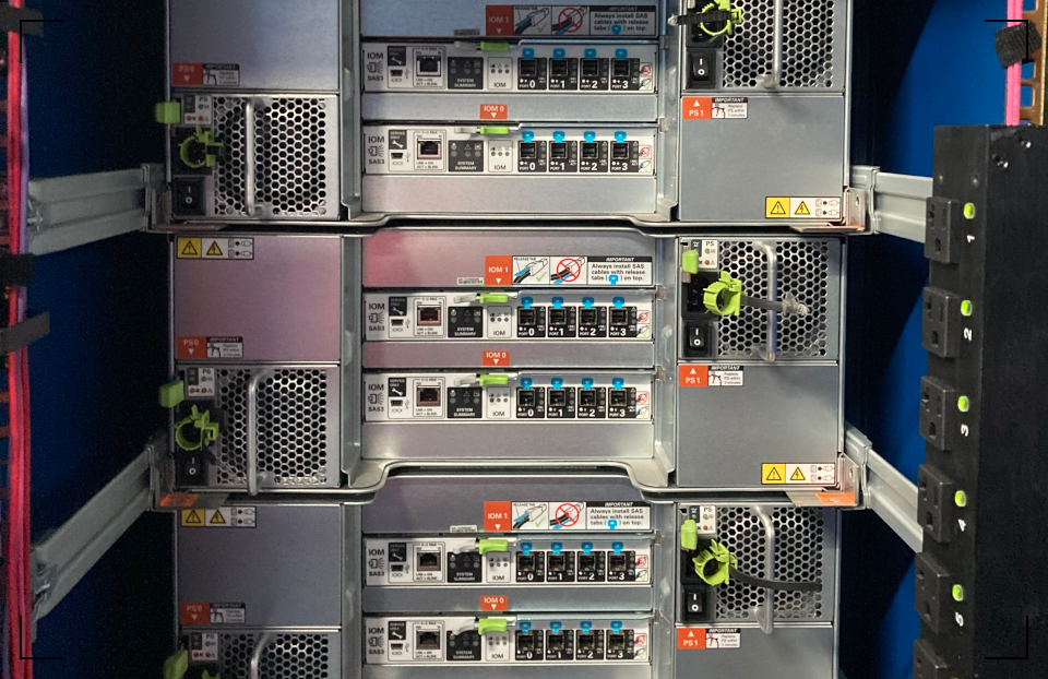
Validation on spec baselines can be tedious, but anyway... the DE3-24C and DE3-24P have very shiny and well made Dual-Redundant IOMs with 4x SAS3 SFF-8643 connectors.
Specs for our SAS3 Fabric with DE3-24 Shelves
- One SAS-3 lane (PHY): 12 Gbit/s ⇒ 1.5 GB/s (raw line-rate, decimal GB)
- External SAS x4 port connector: 4 PHY × 12 Gbit/s ⇒ 48 Gbit/s ⇒ 6 GB/s
- Each DE3-24{C/P} has 2× IOM, with each IOM having 4× SFF-8643 ports
| Item | Value | Notes |
|---|---|---|
| SAS-3 lane rate | 12 Gbit/s | per PHY |
| 1 PHY raw | 1.5 GB/s | 12/8 |
| 1 x4 port raw | 6 GB/s | 4 PHY × 1.5 |
| Shelf fabric cap | 12N GB/s | dual-IOM |
| 10-shelf fabric cap | 120N GB/s | 10 shelves |
| N active x4 ports per IOM | Per-shelf fabric cap (GB/s) | 10-shelf fabric cap (GB/s) |
|---|---|---|
| 1 | 12 | 120 |
| 2 | 24 | 240 |
| 3 (N+1 on 4-port IOM) | 36 | 360 |
| 4 (no spare) | 48 | 480 |
Drive Specs - Seagate EXOS & Oracle SSD
| Drive | Metric | Value |
|---|---|---|
| Seagate Exos ST24000NM007H (24TB HDD) | Max sustained OD (MB/s) | 285 |
| Seagate Exos Mach.2 ST18000NM0272 (18TB HDD) | Max sustained OD (MB/s) | 554 |
| Mach.2 ST18000NM0272 | 4K random @ QD16 (IOPS) | 304 read / 560 write |
| Oracle 7.68TB RI SAS-3 SSD | Seq (MB/s) | 2150 read / 1980 write |
| Oracle 7.68TB RI SAS-3 SSD | 4K random (IOPS) | 450k read / 95k write |
Scenario A – Maximum RAW Block Space
Before going into the theoretical weeds, let's look at some per-shelf media limits.
1) Oracle DE3-24P shelf w/ 24TB Spinners: 24 × 285 MB/s = 6.84 GB/s (media-limited)
2) Oracle DE3-24C shelf w/ SSDs:
- Read: 24 × 2150 MB/s = 51.60 GB/s → capped by fabric at 36 GB/s (N=3)
- Write: 24 × 1980 MB/s = 47.52 GB/s → capped by fabric at 36 GB/s (N=3)
| Tier | Shelves | Per-shelf effective (GB/s) | Tier aggregate (GB/s) |
|---|---|---|---|
| DE3-24P (24× 24TB HDD) | 8 | 6.84 | 54.72 |
| DE3-24C (24× 7.68TB SSD) | 2 | 36.00 (fabric-capped) | 72.00 |
| Total (10 shelves) | 10 | — | 126.72 |
Scenario B: Maximum Performance
Hardware has limits, and we're looking at 8× DE3-24P w/ 18TB Mach.2 HDD + 2× DE3-24C w/ 7.68TB SSD (N=3)
Aggregate sequential bandwidth (N=3)
- Mach.2 18TB HDD shelf: 24 × 554 MB/s = 13.296 GB/s (media-limited; below 36 GB/s fabric cap)
- SSD shelf: remains fabric-capped at 36 GB/s read and write (N=3)
| Tier | Shelves | Per-shelf effective (GB/s) | Tier aggregate (GB/s) |
|---|---|---|---|
| DE3-24P (24× Mach.2 HDD) | 8 | 13.296 | 106.368 |
| DE3-24C (24× 7.68TB SSD) | 2 | 36.000 (fabric-capped) | 72.000 |
| Total (10 shelves) | 10 | — | 178.368 |
Aggregate Random R/W 4K IOPS (N=3)
Fabric-derived 4K IOPS cap per shelf (upper bound):
36 GB/s @ 4KB = approx 8.79M IOPS
- SSD shelf
- Read: 24 × 450k = 10.8M IOPs → capped to 8.79M IOPs
- Write: 24 × 95k = 2.28M IOPs → media-limited (below fabric cap)
- Mach.2 HDD shelf (4K @ QD16)
- Read: 24 × 304 = 7,296 IOPs
- Write: 24 × 560 = 13,440 IOPs
| Tier | Aggregate Read IOPs | Aggregate Write IOPs |
|---|---|---|
| 8× DE3-24P (Mach.2 HDD shelves) | 58,368 | 107,520 |
| 2× DE3-24C (SSD shelves) | 17,580,000 | 4,560,000 |
| Total (10 shelves) | 17,638,368 | 4,667,520 |
Let's See the Deltas!
What's "a delta"? Sometimes it's the headwaters of a bay, where the river distributes across a flood-plane into many separately-unified channels, eventually giving way to deeper waters and.... no no not that kind.
Delta as a value in storage is often used as a marker to show the differential of two functions which indicates directional change. At least, that's what comes from my brain while I sit here having an ice cream sandwich, but it has some alternate terminology which applies irrespective of ice cream hour:
Delta uppercase Δ, lowercase δ
Uppercase: a change of any changeable quantity
Lowercase: the central difference for a function
~ The discriminant of a polynomial equation or symmetric difference of two sets
~ The determinant of the matrix of coefficients of a set of linear equations
Scenario B vs Scenario A (with N=3)
- Total sequential BW: 126.72 → 178.368 GB/s (increase +51.648 GB/s)
- Primary determinant: per-shelf BW 6.84 → 13.296 GB/s (Mach.2 dual-actuator).
- SSD tier remains fabric-capped at 36 GB/s per SSD shelf under N=3; increasing N (or adding more independent uplinks with additional HBAs) is what changes that cap.
- Faster array = less space @ higher IOPs and BW == 178 GB/s @ 3.8PB
- Larger array = more space @ lower IOPs and BW == 126 GB/s @ 4.9PB
Equations w/ decimal units: 1 TB = 1000 GB
- jaja usually we work in 1024 (but I'm tired today, so not right now)
t_1TB(s)      = 1000 / BW_GBps
t_full(s)     = (Capacity_TB * 1000) / BW_GBps
t_full(hours) = t_full(s) / 3600
BW_density    = BW_GBps / Capacity_TB   (GB/s per TB)
              = 1000 * BW_density       (MB/s per TB)
| Metric | Faster array | Larger array |
|---|---|---|
| Bandwidth (GB/s) | 178 | 126 |
| Capacity (TB) | 3824 | 4976 |
| Time per 1 TB (s) | 5.62 | 7.94 |
| Full sweep time (h) | 5.97 | 10.97 |
| BW density (GB/s per TB) | 0.04655 | 0.02532 |
| BW density (MB/s per TB) | 46.55 | 25.32 |
| Density ratio (faster/larger) | 1.84× | — |
So... what's the answer? More, Faster?
Is bigger is better? Sometimes. Sometimes you need it faster. Sometimes you want both.